Modeling
This document describes the carculator_truck model, assumptions
and inventories as exhaustively as possible.
carculator_truck is an open-source Python library. Its code is publicly
available via its Github repository. You can also download an examples notebook, that guides new users into performing life cycle analyses.
Overview of carculator_truck modules
The main module model.py builds the vehicles and delegates the calculation of motive and auxiliary energy, noise, abrasion and exhaust emissions to satellite modules. Once the vehicles are fully characterized, the set of calculated parameters are passed to inventory.py which derives life cycle inventories and calculates life cycle impact indicators. Eventually, these inventories can be passed to export.py to be exported to various LCA software.
Vehicle modelling
The modelling of vehicles along powertrain types, time and size classes is described in this section. It is also referred to as foreground modelling.
Powertrain types
carculator_truck can model the following powertrain types:
Diesel-run internal combustion engine vehicle (ICEV-d)
Gas-run internal combustion engine vehicle (ICEV-g)
Diesel-run hybrid electric vehicle (HEV-d)
Diesel-run plug-in hybrid electric vehicle (PHEV-d)
Battery electric vehicle (BEV) with charging at depot
Fuel cell electric vehicle (FCEV)
Size classes
Several size classes are available for each powertrain type. They refer to the maximum permissible gross weight of the vehicle (e.g., 32 tons). In addition, several application-specific designs are available for each powertrain-size class combination, namely: Urban delivery, Regional delivery and Long haul. They are associated with a given range autonomy: 150 km, 400 km and 800 km, respectively. This is particularly relevant for sizing the onboard energy storage unit. Some powertrain-size class-application combinations are not commercially available or technologically mature and are therefore not considered.
Battery electric vehicles are not considered for years prior to
2020. Additionally, carculator_truck may not find a solution for
regional delivery and long haul use in 2020, as the volumetric
density of batteries does not currently allow a range autonomy superior
to 400 km without significantly sacrificing the cargo carrying capacity.
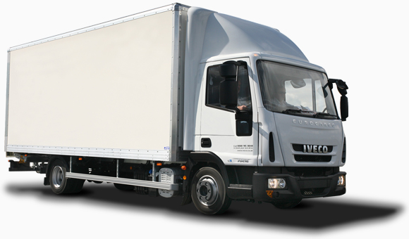
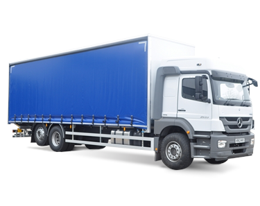
carculator_truck defines seven size classes, namely:
3.5t
7.5t
18t
26t
32t
40t
60t
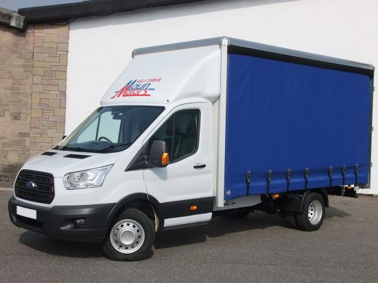
Example of 3.5t truck, rigid, 2 axles, box body and 7.5t truck, rigid, 2 axles, box body
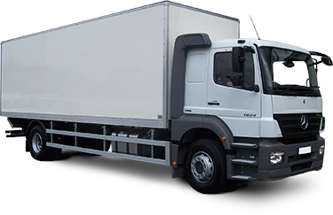
Example of 18t truck, rigid, 2 axles, box body and 26t truck, rigid, 3 axles, box body
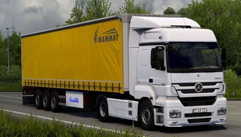
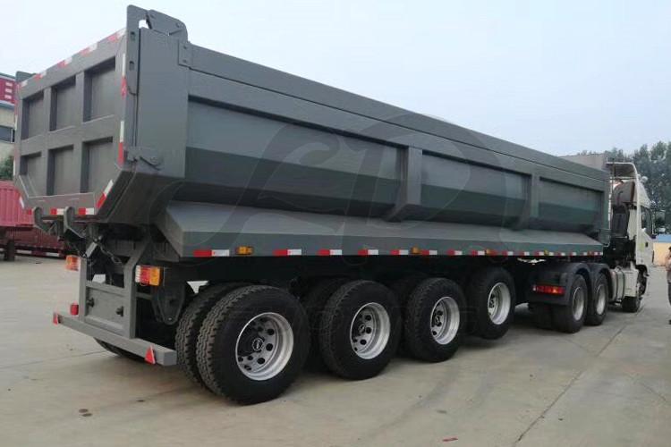
Example of 32t truck, semi-trailer, 2+3 axles, curtain-sider and 40t truck, tipper-trailer, 2+4 axles
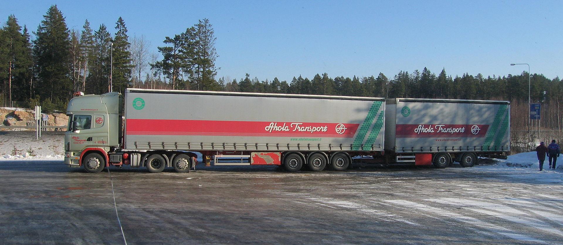
Example of 60t truck, semi-trailer + trailer, 2+4+2 axles, curtain-sider
Manufacture year and emission standard
For ICE vehicles, several emission standards are considered. For simplicity, it is assumed that the vehicle manufacture year corresponds to the registration year. Those are presented in Table 1.
Start of registration |
End of registration (incl.) |
Manufacture year in this study |
|
|---|---|---|---|
EURO-3 |
2000 |
2004 |
2002 |
EURO-4 |
2005 |
2007 |
2006 |
EURO-5 |
2008 |
2012 |
2010 |
EURO-6 |
2013 |
2020 |
Modelling considerations applicable to all vehicle types
Sizing of the base frame
The sizing of the base frame is based on p. 17-19 of [Nikolas and others, 2015]. Detailed weight composition is obtained for a 12t rigid truck and a 40t articulated truck. Curb mass and payload are obtained for all size classes, the rest being adjusted function of the gross mass. The masses of the vehicles and their subsystems are detailed in Table 2. These truck models have 2010 as baseline year. A 2% and 5% weight reduction factors are applied on on rigid and articulated trucks respectively, as indicated in the same report.
The following components are common to all powertrains:
Frame
Suspension
Brakes
Wheels and tires,
Electrical system
Transmission
Other components
Rigid truck, 3.5t |
Rigid truck, 7.5t |
Rigid truck, 12t |
Rigid truck, 18t |
Rigid truck, 26t |
Articulated truck, 32t |
Articulated truck, 40t |
Articulated truck, 60t |
||
|---|---|---|---|---|---|---|---|---|---|
Type |
rigid, 2 axles, box body |
rigid, 2 axles, box body |
rigid, 2 axles, box body |
rigid, 2 axles, box body |
rigid, 3 axles, box body |
semi-trailer, 2+3 axles, curtain-sider |
semi-trailer, 2+4 axles, curtain-sider |
semi-trailer + trailer, 2+4+2 axles, curtain-sider |
|
in kilograms |
Gross weight |
3500 |
7500 |
12000 |
18000 |
26000 |
32000 |
40000 |
60000 |
Powertrain |
Engine system |
151 |
324 |
518 |
777 |
1122 |
899 |
1124 |
1686 |
Coolant system |
11 |
23 |
37 |
56 |
80 |
112 |
140 |
210 |
|
Fuel system |
14 |
29 |
47 |
71 |
102 |
64 |
80 |
120 |
|
Exhaust system |
44 |
94 |
150 |
225 |
325 |
176 |
220 |
330 |
|
Transmission system |
83 |
177 |
283 |
425 |
613 |
446 |
558 |
837 |
|
Electrical system |
24 |
52 |
83 |
125 |
180 |
212 |
265 |
398 |
|
Chassis system |
Frame |
120 |
256 |
410 |
615 |
888 |
2751 |
3439 |
5159 |
Suspension |
310 |
665 |
1064 |
1596 |
2000 |
2125 |
2656 |
3984 |
|
Braking system |
24 |
52 |
83 |
125 |
180 |
627 |
784 |
1176 |
|
Wheels and tires |
194 |
416 |
665 |
998 |
1100 |
1138 |
1422 |
2133 |
|
Cabin |
Cabin |
175 |
375 |
600 |
900 |
1300 |
922 |
1153 |
1730 |
Body system/trailer |
583 |
1250 |
2000 |
3000 |
4333 |
1680 |
2100 |
3150 |
|
Other |
119 |
256 |
409 |
614 |
886 |
847 |
1059 |
1589 |
|
Curb mass, incl. Trailer |
1852 |
3968 |
6349 |
9524 |
13110 |
12000 |
15000 |
22500 |
|
Payload |
1648 |
3532 |
5651 |
8477 |
12890 |
20000 |
25000 |
37500 |
Other use and size-related parameters
HBEFA 4.1 is used as a source to estimate the calendar and kilometric lifetime values for European diesel trucks. Those are presented in Table 3.
Size class in this study |
3.5t |
7.5t |
18t |
26t |
32t |
40t |
Source |
|
|---|---|---|---|---|---|---|---|---|
HBEFA vehicle segments |
Unit |
RigidTruck <7,5t |
RigidTruck 7,5-12t |
RigidTruck >14-20t |
RigidTruck >26-28t |
TT/AT >28-34t |
TT/AT >34-40t |
|
Yearly mileage at Year 1 |
Km |
32’526 |
47’421 |
37’602 |
69’278 |
31’189 |
118’253 |
HBEFA 4.1 |
Relative annual decrease in annual mileage |
5.50% |
7% |
Estimated from HBEFA 4.1 |
|||||
Calendar lifetime |
Year |
12 |
12 |
8 |
Estimated from HBEFA 4.1 |
|||
Kilometric lifetime |
km |
272’000 |
397’000 |
315’000 |
580’000 |
227’000 |
710’000 |
Calculated from the rows above |
Average loads for European trucks for long haul use are from the TRACCS road survey data for the EU-28 [G. and others, 2013]. We differentiate loads across driving cycles. To do so, we use correction factors based on the representative loads suggested in the Annex I of European Commission regulation 2019/1242. Such average loads are presented in Table 4.
Size class |
3.5t |
7.5t |
18t |
26t |
32t |
40t |
||
|---|---|---|---|---|---|---|---|---|
Cargo carrying capacity |
ton |
~1.3 |
~3.5 |
~10.1 |
~17.0 |
~20.1 |
~25.5 |
Manufacturers’ data. |
Cargo mass (urban delivery) |
ton |
0.75 |
1.75 |
2.7 |
6.3 |
8.75 |
8.75 |
Long haul cargo mass, further corrected based on EC regulation 2019/1242 |
Cargo mass (regional delivery) |
ton |
0.75 |
1.75 |
3.2 |
6.3 |
10.3 |
19.3 |
Long haul cargo mass, further corrected based on EC regulation 2019/1242 |
Cargo mass (long haul) |
ton |
1.13 |
2.63 |
7.4 |
13.4 |
13.8 |
13.8 |
TRACCS (Papadimitriou et al. 2013) for EU28 |
The user can however easily change these values.
Other size-related parameters are listed in Table 5. Some of them have been obtained and/or calculated from manufacturers’ data, which is made available in the Annex A-C of this report.
Size class in this study |
3.5t |
7.5t |
18t |
26t |
32t |
40t |
Source |
|
|---|---|---|---|---|---|---|---|---|
Number of axles |
unit |
2 |
2 |
2 |
3 |
5 |
6 |
Manufacturers’ data. |
Rolling resistance coefficient |
unitless |
.0055 |
.0055 |
.0055 |
.0055 |
.0055 |
.0055 |
(Meszler et al. 2018) |
Frontal area |
square meter |
4.1 |
5.3 |
7.5 |
7.5 |
10 |
10 |
Manufacturers’ data. |
Passengers occupancy |
unit |
1 |
1 |
1 |
1 |
1 |
1 |
Inferred from Mobitool factors v.2.1 values |
Average passenger mass |
kilogram |
75 |
Standard assumption |
The user can however easily change these values.
Time-dependent parameters
Several parameters that affect the performances of trucks (e.g., drag coefficient, etc.) are time-dependent, and based on various projections found in the literature. Table 6 lists some of them.
Size class in this study |
2000 |
2010 |
2020 |
2030 |
2040 |
2050 |
Source |
|
|---|---|---|---|---|---|---|---|---|
Aerodynamic drag |
unitless |
0.55 |
0.5 |
0.47 |
0.45 |
0.43 |
0.4 |
ICCT, 2021 |
Rolling resistance coefficient |
unitless |
.0055 |
.0055 |
.0055 |
.004 |
.004 |
.004 |
ICCT, white paper, 2018, assumption |
NMC battery cycling life |
unit |
3000 |
3000 |
3000 |
4000 |
4000 |
4000 |
(Preger et al. 2020), assumption |
NMC cell energy density |
kWh/kg |
0.05 |
0.1 |
0.2 |
0.3 |
0.4 |
0.5 |
(Qiao et al., 2020, ScienceDaily, 2022) |
Fuel cell power density |
mW/cm2 |
350 |
400 |
450 |
450 |
500 |
600 |
(Cox et al. 2020) |
Modelling approach applicable to internal combustion engine vehicles
Traction energy
The traction energy for medium- and heavy-duty trucks is calculated based on the driving cycles for trucks provided by VECTO. Simulations are run in VECTO with trucks modeled as closely as possible to those of this study, to obtain performance indicators along the driving cycle (e.g., speed and fuel consumption, among others).
The calculation of the total resistance to overcome at the wheel level is the sum of the following resistances:
The vehicle inertia, calculated as acceleration * driving mass
The rolling resistance, calculated as driving mass * rolling resistance coefficient * gravity
The aerodynamic drag, calculated as frontal area * aerodynamic drag coefficient * air density * speed^2 / 2
The gradient resistance, calculated as driving mass * gravity * sin(gradient)
As well as the resistance from braking, calculated as the force from the vehicle inertia when negative.
Figure 1 shows the contribution of each type of resistance as calculated by
carculator_truck for the first hundred seconds of the “Urban delivery” driving cycle, for an 18t diesel truck.
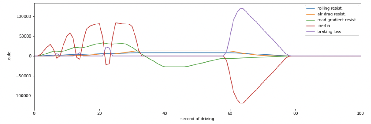
Figure 1: Resistance components at wheels level for the first hundred seconds of the “Urban delivery” driving cycle, for an 18t diesel truck.
Figure 2 shows the first two hundred seconds of the “Urban delivery” driving cycle. It distinguishes the target speed from the actual speed managed by the different vehicles. The power-to-mass ratio influences the extent to which a vehicle manages to comply with the target speed.
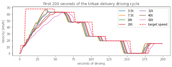
Figure 2: VECTO’s “Urban delivery” driving cycle (first two hundred seconds)
For regional delivery and long haul use, the “Regional delivery” and “Long haul” driving cycles of VECTO are used, respectively. They contain less stops and fewer fluctuations in terms of speed levels. The “Long haul” driving cycle has a comparatively higher average speed level and lasts much longer. Figure 3 shows the first two hundred seconds of the “Long haul” driving cycle.
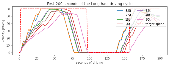
Figure 3: VECTO’s “Long haul” driving cycle (first two hundred seconds)
Table 7 shows a few parameters about the three driving cycles considered. Value intervals are shown for some parameters as they vary across size classes.
Note
Important remark: unlike the modeling of passenger cars, the vehicles are designed in order to satisfy a given range autonomy. The range autonomy specific to each driving cycle is specified in the last column of Table 7. This is particularly relevant for battery electric vehicles: their energy storage unit is sized to allow them to drive the required distance on a single battery charge. While this also applies for other powertrain types (i.e., the diesel fuel tank or compressed gas cylinders are sized accordingly), the consequences in terms of vehicle design are not as significant. The required range autonomy shown in Table 7 is not defined by VECTO, but set as desirable range values by the authors of the software. The target range autonomy can easily be changed by the user.
Driving cycle |
Average speed [km/h] |
Distance [km] |
Driving time [s] |
Idling time [s] |
Mean positive acceleration [m.s2] |
Required range autonomy [km] |
|---|---|---|---|---|---|---|
Urban delivery |
9.9 - 10.7 |
28 |
~10’000 |
614 - 817 |
0.26 - 0.55 |
150 |
Regional delivery |
16.5 - 17.8 |
26 |
~5’500 |
110 - 220 |
0.21 - 0.52 |
400 |
Long haul |
19.4 - 21.8 |
108 |
~19’400 |
240 - 868 |
0.13 - 0.54 |
800 |
The energy consumption model is similar to that of passenger cars: different resistances at the wheels are calculated, after which friction-induced losses along the drivetrain are considered to obtain the energy required at the tank level.
VECTO’s simulations are used to calibrate the engine and transmission efficiency of diesel trucks. Similar to the modeling of buses, the relation between the efficiency of the drivetrain components (engine, gearbox) and the power load-to-peak-power ratio is used.
Indeed, once the power requirement at the wheel level for each second is known
(and validated), inefficiencies from the transmission line and the engine need
to be accounted for. Here again, second-by-second data from VECTO simulations are used.
VECTO uses a complex gearshift model combined with an engine-specific torque map that
are too complex to be implemented in carculator_truck. Instead, the relation between
transmission and engine efficiency on one end, and the relative power load (i.e.,
power load over the rated power output of the engine) on the other end, is used.
Such relations are shown in Figure 4, for a 40t diesel truck, where the efficiency of the
drivetrain (left) and engine (right) in relation to the power load is plotted for
each second of the “Urban delivery” driving cycle, with a loading factor of 100%.
For example, Figure 4.a shows that the transmission efficiency (that is, from the
wheels to the output shaft of the engine) is close to 85% at a power load of 20%.
In fact, most of the time when the truck is driving, the transmission operates at above
80% efficiency. Similarly, Figure 4.b shows that the peak engine efficiency is reached
at about 40% power load, after which it remains more or less constant.
A curve is fitted on the data points (red line). Using such fit removes some of
the complexity considered in VECTO, depicted here by the measurements that deviate
for the red curve. Nevertheless, it allows obtaining a reasonable estimate of
the efficiency of these drivetrain components.
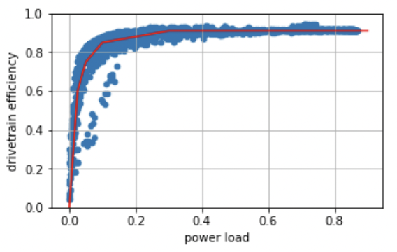
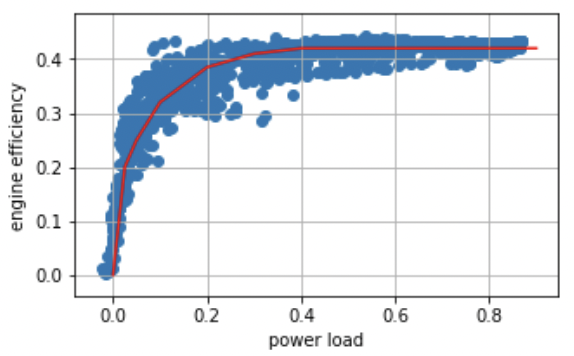
Relation between transmission and engine efficiency on one end, and the relative power load on the other end
Such calibration exercise with VECTO for the diesel-powered 40t truck is
shown below, against the “Urban delivery” driving cycle. After
calibration, the tank-to-wheel energy consumption value obtained from
VECTO and from carculator_truck for diesel-powered trucks differ by
less than 1 percent over the entire driving cycle.
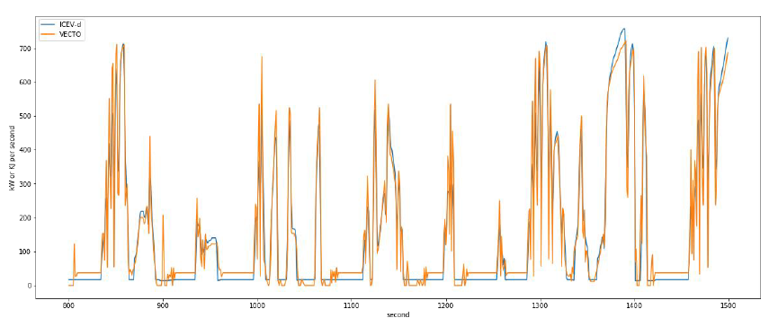
Figure 5: Calibration of carculator_truck energy model against VECTO simulations for a 40t articulated truck diesel truck (first 1’500 seconds shown)
Unfortunately, VECTO does not have a model for compressed gas-powered trucks. The calibrated model for diesel-powered buses is used and a penalty factor of 10% is applied, based on findings from a working paper from the ICCT [Ragon and Rodríguez, 2021] showing that compressed gas-powered trucks have an engine efficiency between 8 to 13% lower than that of diesel-powered trucks.
Engine downsizing
Such approach allows also reflecting the effect of engine downsizing. As the relative power load observed during the driving cycle is higher as the rated maximum power output of the engine is reduced, it operates at higher efficiency levels. Figure 6 compares the engine efficiency between a conventional 40t diesel truck and a diesel hybrid truck of similar size, but where the power of the combustion engine is reduced by 25% in favor of an electric motor. This figure confirms that the combustion engine of hybrid-diesel truck (HEV-d) reaches higher efficiency levels. Of course, the difference in efficiency will be more pronounced on driving cycles with transient loads.
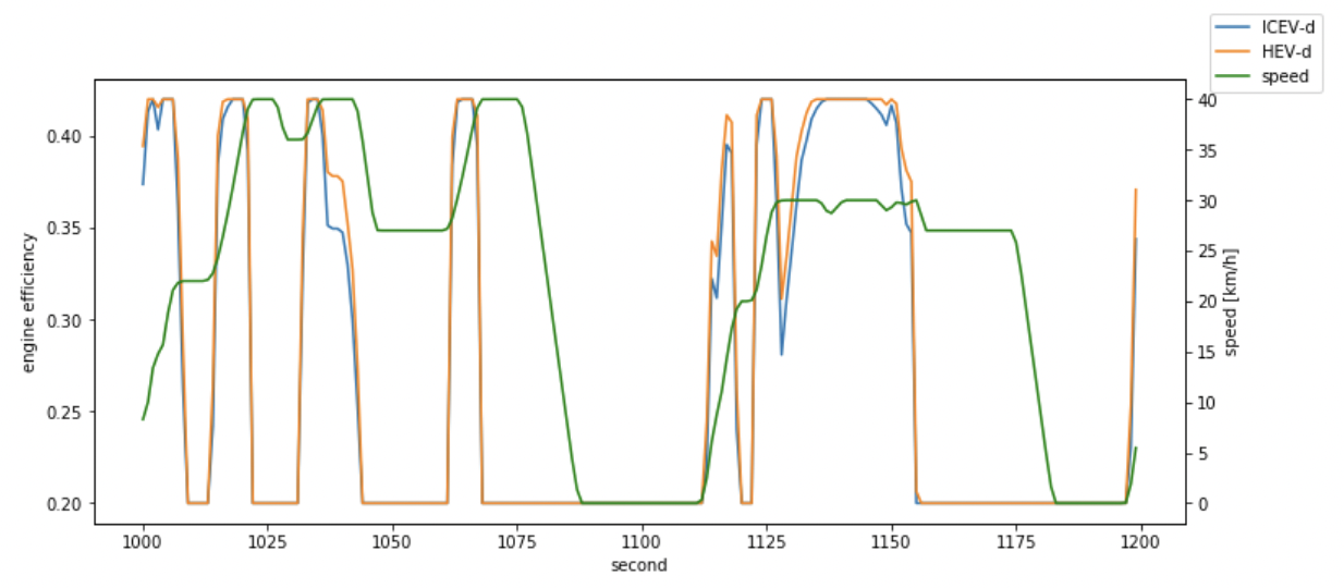
Figure 6: Engine efficiency comparison between a conventional (ICEV-d) and hybrid (HEV-d) 40t diesel truck
Compressed gas trucks
For compressed gas trucks, the energy storage is in a four-cylinder configuration, with each cylinder containing up to 57.6 kg of compressed gas – 320 liters at 200 bar.
The relation between the mass of compressed gas and the cylinder mass is depicted in Figure 7. This relation is based on manufacturers’ data – mainly from [Trucks, n.d., QTWW, 2021].
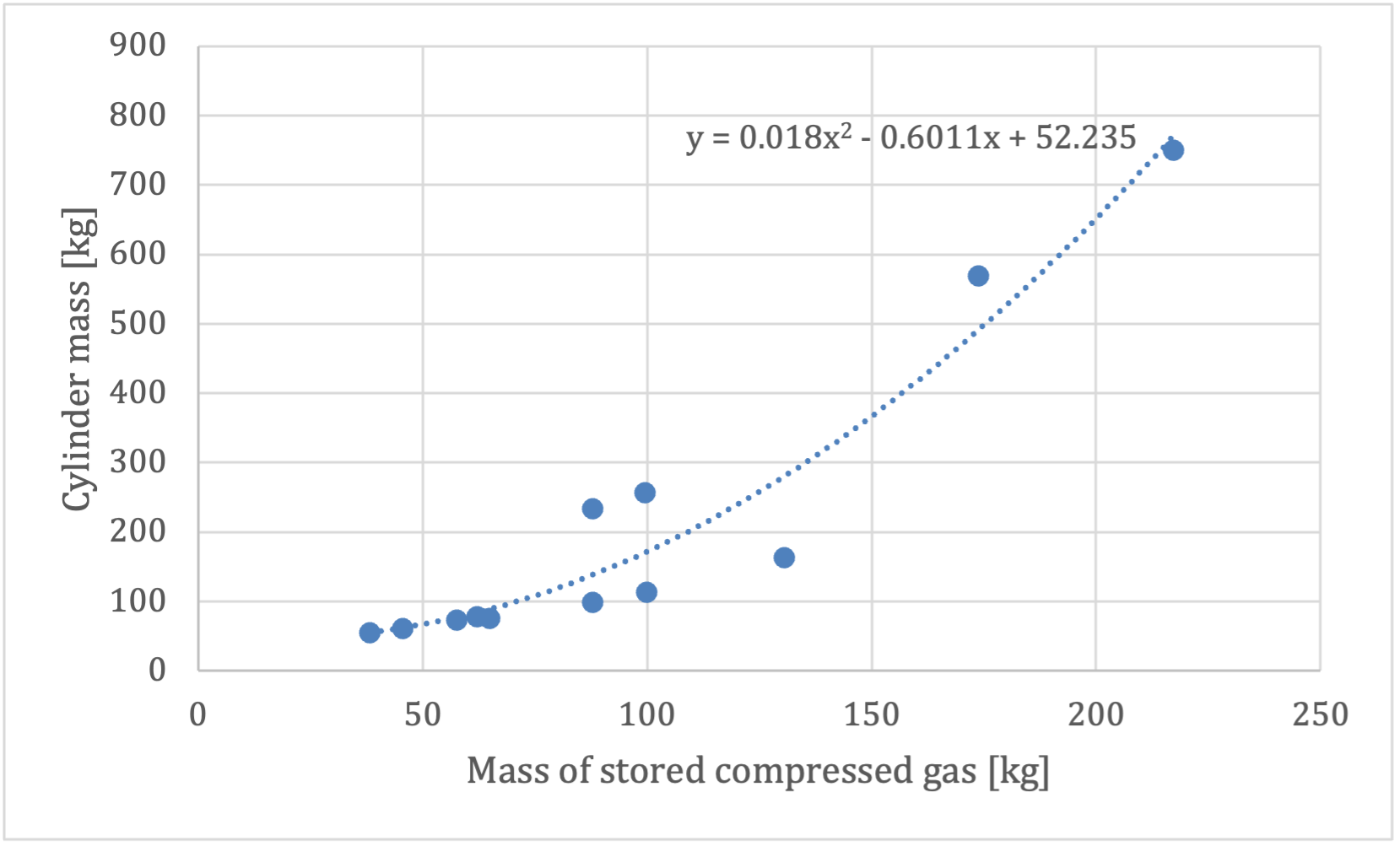
Figure 7: Relation between mass of stored compressed gas and cylinder mass
Inventories for a Type II 200 bar compressed gas tank, with a steel liner, are from [Daniele and others, 2021].
Exhaust emissions
Other pollutants
Emission factors for CO2 and SO2 are detailed in Table 8 - Table 9. Biofuel shares in the fuel blend are detailed in Table 10.
A number of fuel-related emissions other than CO2 or SO2 are also considered.
For trucks, two sources source of emissions are considered:
Exhaust emissions: emissions from the combustion of fuel during operation. Their concentration relates to the fuel consumption and the emission standard of the vehicle.
Non-exhaust emissions: abrasion emissions such as brake, tire and road wear, but also emissions of refrigerant and noise.
For exhaust emissions, factors based on the fuel consumption are derived by comparing emission data points for different traffic situations (i.e., grams emitted per vehicle-km) in free-flowing driving conditions, with the fuel consumption corresponding to each data point (i.e., MJ of fuel consumed per km), as illustrated in for a diesel-powered engine. The aim is to obtain emission factors expressed as grams of substance emitted per MJ of fuel consumed, to be able to model exhaust emissions of trucks of different sizes, masses, operating on different driving cycles and with different load factors.
Note
Important remark: the degradation of anti-pollution systems for EURO-6 diesel trucks (i.e., catalytic converters) is accounted for as indicated by HBEFA 4.1, by applying a degradation factor on the emission factors for NOx. These factors are shown in Table 8 for trucks with a mileage of 890’000 km. Since the trucks in this study have a kilometric lifetime of 180-700’000 km, degradation factors are interpolated linearly (with a degradation factor of 1 at Km 0). The degradation factor corresponding to half of the vehicle kilometric lifetime is used, to obtain a lifetime-weighted average degradation factor.
Degradation factor at 890’000 km |
|
|---|---|
NOx |
|
EURO-6 |
1.3 |
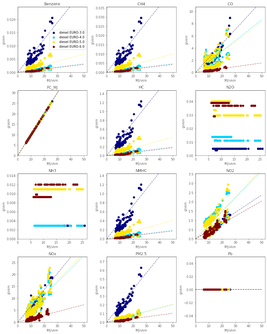
Figure 8: Relation between emission factors and fuel consumption for a diesel-powered truck for a number of “urban” and “rural” traffic situations for different emission standards.
Using these fuel-based emission factors, emissions for each second of the driving cycle for each substance are calculated.
To confirm that such approach does not yield kilometric emissions too
different from the emission factors per vehicle-kilometer proposed by
HBEFA 4.1, Figure 9 compares the emissions obtained by
carculator_truck using VECTO’s “Urban delivery” driving cycle over 1
vehicle-km (red dots) for a 18t rigid truck with the distribution of the
emission factors across different “urban” traffic situations (green
box-and-whiskers) given by HBEFA 4.1, as well as its weighted average
(yellow dots) for different emission standards for a rigid truck with a
gross mass of 14-20 tons.
There is some variation across HBEFA’s urban traffic situations, but the
emissions obtained remain, for most substances, within the 50% of the
distributed HBEFA values across traffic situations. Special attention
must be paid to EURO-III vehicles, for which emissions tend to be
slightly over-estimated by carculator_truck. The comparison between
the model’s emission results for the regional and long-haul driving
cycles using trucks of different size classes and HBEFA’s emission
factors for “rural” and “motorway” traffic situations shows a similar
picture.
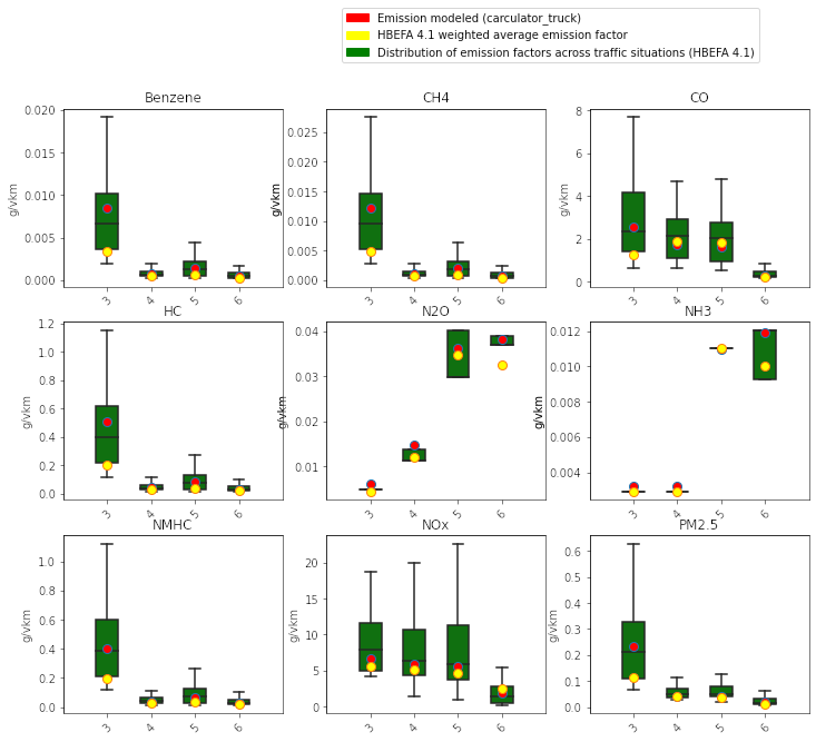
Figure 9: Validation of the exhaust emissions model with the emission factors provided by HBEFA 4.1 for medium-duty trucks in traffic urban and rural situations, for different levels of service.
Note
Box-and-whiskers: distribution of HBEFA’s emission factors (box: 50% of the distribution, whiskers: 90% of the distribution). Yellow dots: traffic situations-weighted average emission factors.
Red dots: modeled emissions calculated by carculator_truck with the “Urban delivery” driving cycle for an 18t rigid truck, using the relation between fuel consumption and amounts emitted.
Modelling approach applicable to electric vehicles
Traction energy
Electric vehicles
VECTO does not have a model for battery or fuel cell electric buses that can be used. Therefore, similarly to the modeling of buses, static engine and drivetrain efficiency values are used. These values are based on [Schwertner and Weidmann, 2016] and are presented in Table 9-Table 10.
Eff. of subsystem |
Fuel cell bus |
BEV bus |
Trolleybus |
Fuel tank |
0.98 |
||
Energy storage |
0.92 |
||
Fuel cell stack |
0.55 |
||
Converter |
0.98 |
||
Rectifier |
|||
Inverter |
0.98 |
0.98 |
0.98 |
Electric motor |
0.93 |
0.93 |
0.93 |
Reduction gear |
0.95 |
0.95 |
0.95 |
Drive axle |
0.94 |
0.94 |
0.94 |
Total |
0.44 |
0.73 |
0.81 |
Eff. of subsystem |
Fuel cell bus |
BEV bus |
BEV-motion |
Drive axle |
0.94 |
0.94 |
0.94 |
Reduction gear |
0.95 |
0.95 |
0.95 |
Electric motor |
0.93 |
0.93 |
0.93 |
Rectifier |
0.98 |
0.98 |
0.98 |
Converter |
0.98 |
0.98 |
|
Energy storage |
0.85 |
0.85 |
0.85 |
Converter |
0.98 |
0.98 |
|
Inverter |
0.98 |
0.98 |
0.98 |
Electric motor |
0.93 |
0.93 |
0.93 |
Reduction gear |
0.95 |
0.95 |
0.95 |
Drive axle |
0.94 |
0.94 |
0.94 |
Total |
0.54 |
0.54 |
0.56 |
Energy storage
Battery electric trucks
Battery electric vehicles can use different battery chemistry (Li-ion NMC, Li-ion LFP, Li-ion NCA and Li-LTO) depending on the manufacturer’s preference or the location of the battery supplier. Unless specified otherwise, all battery types are produced in China, as several sources, among which BloombergNEF [Henze, 2020], seem to indicate that more than 75% of the world’s cell capacity is manufactured there. Accordingly, the electricity mix used for battery cells manufacture and drying, as well as the provision of heat are assumed to be representative of the country (i.e., the corresponding providers are selected from the LCI background database). The battery-related parameters considered in this study are shown in Table 11. For LFP batteries, “blade battery” or “cell-to-pack” battery configurations are considered, as introduced by CATL [Xinhua, 2019] and BYD [Mark, 2020], two major LFP battery suppliers in Asia. This greatly increases the cell-to-pack ratio and the gravimetric energy density at the pack level.
Overall, the gravimetric energy density values at the cell and system levels presented in Table 11 are considered conservative: some manufacturers perform significantly better than the average, and these values tend to change rapidly over time, as it is being the focus of much R&D.
The sizing of energy storage for BEV trucks is sensitive to the required range autonomy, which is specific to each driving cycle (or defined by the user).
Note
Important remark: technically speaking carculator_truck will model
all trucks. However, if a vehicle has an energy storage unit mass
leading to a reduction in the cargo carrying capacity beyond a
reasonable extent, it will not be processed for LCI quantification. This
is the reason why battery electric trucks used for long haulage (i.e.,
with a required range autonomy of 800 km) are not considered before ~2030.
The expected battery lifetime (and the need for replacement) is based on the battery expected cycle life, based on theoretical values given by [Dietmar and others, 2018] as well as some experimental ones from [Yuliya and others, 2020]. Although the specifications of the different battery chemistry are presented in Table 11, they are also repeated in Table 12.
Lithium Nickel Manganese Cobalt Oxide (LiNiMnCoO2) — NMC[1] |
Lithium Iron Phosphate(LiFePO4) — LFP |
Lithium Nickel Cobalt Aluminum Oxide (LiNiCoAlO2) — NCA |
Source |
|
|---|---|---|---|---|
Cell energy density [kWh/kg] |
0.2 |
0.15 |
0.23 |
|
Cell-to-pack ratio |
0.6 |
0.8 |
0.6 |
|
Pack-level gravimetric energy density [kWh/kg] |
0.12 |
0.12 |
0.14 |
Calculated from the two rows above |
Share of cell mass in battery system [%] |
60 to 80% (others, depending on chemistry, see third row above) |
|||
Maximum state of charge [%] |
100% |
100% |
100% |
|
Minimum state of charge [%] |
20% |
20% |
20% |
|
Cycle life to reach 20% initial capacity loss (80%-20% SoC charge cycle) |
2’000 |
7’000+ |
1’000 |
|
Corrected cycle life |
3’000 |
7’000 |
1’500 |
Assumption |
Charge efficiency |
85% |
[Schwertner and Weidmann, 2016] for buses and trucks. [Rantik, 1999] for battery charge efficiency when ultra-fast charging. |
||
Discharge efficiency |
88% |
The default NMC battery cell corresponds to a so-called NMC 6-2-2 chemistry: it exhibits three times the mass amount of Ni compared to Mn, and Co, while Mn and Co are present in equal amount. Development aims at reducing the content of Cobalt and increasing the Nickel share. The user can also select NMC-1-1-1 or NMC-8-1-1.
Note
Important remark: the battery cell energy density is not the same as the battery pack energy density. The latter is the product of the cell energy density and the cell-to-pack ratio.
Changing the cell chemistry affects the caurb mass of the vehicle and its cargo carrying capacity (since the range autonomy required remains unchanged).
Lithium Nickel Manganese Cobalt Oxide (LiNiMnCoO2) — NMC[1] |
Lithium Iron Phosphate(LiFePO4) — LFP |
Lithium Nickel Cobalt Aluminum Oxide (LiNiCoAlO2) — NCA |
Source |
||||
|---|---|---|---|---|---|---|---|
Cell energy density [kWh/kg] |
2020 |
0.2 |
2020 |
0.15 |
2021 |
0.23 |
[BatteryUniversity, 2021, Xiao-Guang and others, 2021, Yu and others, 2020, ScienceDaily, 2022, of Energy Efficiency and Energy, 2020] |
2030 |
0.3 |
2030 |
0.17 |
2030 |
0.31 |
||
2040 |
0.4 |
2040 |
0.19 |
2040 |
0.4 |
||
2050 |
0.5 |
2050 |
0.21 |
2050 |
0.5 |
||
Cell-to-pack ratio |
2020 |
0.6 |
2020 |
0.8 |
2021 |
0.6 |
|
2030 |
0.625 |
2030 |
0.85 |
2030 |
0.625 |
||
2040 |
0.65 |
2040 |
0.9 |
2040 |
0.65 |
||
2050 |
0.65 |
2050 |
0.9 |
2050 |
0.65 |
||
Pack-level gravimetric energy density [kWh/kg] |
2020 |
0.12 |
2020 |
0.12 |
2021 |
0.14 |
Calculated from the two parameters above |
2030 |
0.19 |
2030 |
0.14 |
2030 |
0.19 |
||
2040 |
0.26 |
2040 |
0.17 |
2040 |
0.26 |
||
2050 |
0.33 |
2050 |
0.19 |
2050 |
0.33 |
||
Maximum state of charge [%] |
100% |
100% |
100% |
||||
Minimum state of charge [%] |
20% |
20% |
20% |
||||
Cycle life to reach 20% initial capacity loss (80%-20% SoC charge cycle) |
2’000 |
7’000+ |
1’000 |
||||
Corrected cycle life |
3’000 |
7’000 |
1’500 |
Assumption |
|||
Charge efficiency |
2020 |
85% |
[Brian and others, 2020, Brian and others, 2020] for passenger cars. |
||||
2030 |
86% |
||||||
2040 |
86% |
||||||
2050 |
86% |
||||||
Discharge efficiency |
2020 |
88% |
|||||
2030 |
89% |
||||||
2040 |
89% |
||||||
2050 |
89% |
For trucks, for which the mileage varies across size classes and application types, the number of battery replacements is calculated based on the required number of charge cycles (which is itself conditioned by the battery capacity and the total mileage over the lifetime), in relation with the cycle life of the battery (which differs across chemistry – see Table 11).
Note
Important assumption: The environmental burden associated with the manufacture of spare batteries is entirely allocated to the vehicle use. The number of battery replacements is rounded up.
Given the energy consumption of the vehicle and the required battery
capacity, carculator_truck calculates the number of charging cycles
needed and the resulting number of battery replacements, given the cycle
life of the chemistry used. As discussed above, the expected cycle life is corrected.
Beyond the chemistry-specific resistance to degradation induced by charge-discharge cycles, the calendar aging of the cells for batteries that equip trucks is also considered: regardless of the charging type and cycle life, there is a minimum of one replacement of the battery during the vehicle lifetime.
Table 13 gives an overview of the number of battery replacements assumed for the different electric vehicles in this study.
NMC |
LFP |
NCA |
|
|---|---|---|---|
Medium/heavy duty truck, urban delivery |
1 |
1 |
1 |
Medium/heavy duty truck, regional delivery |
1 |
1 |
1 |
Plugin hybrid trucks
The number of commercial models of plugin hybrid trucks is limited. In this study, plugin hybrid trucks are mostly modeled after Scania’s PHEV tractor [Scania, 2020]. It comes with three 30 kWh battery packs, giving it a range autonomy in battery-depleting mode of 60 km, according to the manufacturer. These specifications in terms of battery capacity are used to model plugin hybrid trucks of different size classes (i.e., roughly based on their respective gross mass).
Knowing the vehicle battery storage capacity and its tank-to-wheel efficiency when powered on battery, it is possible to calculate its resulting range autonomy in battery-depleting mode. Furthermore, it is assumed that, in the context of urban delivery, the truck is used in battery-depleting mode in priority, resorting the combustion mode to complete the driving cycle (i.e., 150 km). This approach is used to calculate the electric utility factor for these vehicles. Energy storage capacities and electric utility factors for plugin hybrid trucks are described in Table 14.
Size class |
Battery capacity |
Range autonomy in battery-depleting mode |
Required range autonomy |
Electric utility factor |
Comment |
|---|---|---|---|---|---|
kWh |
km |
km |
% |
The km driven in combustion mode complete the distance required by the range autonomy. |
|
3.5t |
20 |
50 |
150 |
35 |
|
7.5t |
30 |
47 |
33 |
||
18t |
70 |
50 |
35 |
||
26t |
90 |
45 |
33 |
||
32t |
95 |
45 |
32 |
||
40t |
110 |
48 |
33 |
Fuel cell electric trucks
All fuel cell electric vehicles use a proton exchange membrane (PEM)-based fuel cell system.
Table 15 lists the specifications of the fuel cell stack and system used in carculator_truck.
The durability of the fuel cell stack, expressed in hours, is used to determine
the number of replacements needed – the expected kilometric lifetime of the vehicle
as well as the average speed specified by the driving cycle gives the number
of hours of operation. The environmental burden associated with the manufacture of
spare fuel cell systems is entirely allocated to vehicle use as no reuse channels
seem to be implemented for fuel cell stacks at the moment.
Trucks |
Source |
|
|---|---|---|
Power [kW] |
30 - 140 |
Calculated. |
Fuel cell stack efficiency [%] |
55-58% |
|
Fuel cell stack own consumption [% of kW output] |
15% |
|
Fuel cell system efficiency [%] |
45-50% |
|
Power density [W/cm2 cell] |
0.45 |
For passenger cars, [Simons and Bauer, 2015]. For trucks and buses, the power density is assumed to be half that of passenger cars, to reflect an increased durability. |
Specific mass [kg cell/W] |
1.02 |
|
Platinum loading [mg/cm2] |
0.13 |
|
Fuel cell stack durability [hours to reach 20% cell voltage degradation] |
17’000 |
|
Fuel cell stack lifetime replacements [unit] |
0 - 2 |
Calculated. |
The energy storage unit of fuel cell electric trucks is sized based on the required amount of hydrogen onboard (defined by the required range autonomy). The relation between hydrogen mass and tank mass is derived from manufacturers’ specifications, as shown in Figure 10.
We start from the basis that fuel cell electric trucks are equipped with 650 liters cylinders, which contain 14.4 kg hydrogen at 700 bar, for a (empty) mass of 178 kg. Hence, the requirement in term of tank mass for a long haul fuel cell electric truck that needs 74 kg of hydrogen is 0.19162 + 14.586*14.4 + 10.8 * (74/14.4) = 1’068 kg, excluding the hydrogen mass.
The hydrogen tank is of type IV, a carbon fiber-resin (CF) composite-wrapped single tank system, with an aluminium liner capable of storing 5.6 kg usable hydrogen, weighting 119 kg per unit (of which 20 kg is carbon fiber), which has been scaled up to 178 kg for a storage capacity of 14.4 kg to reflect current models on the market [Quantum, 2019]. The inventories are originally from [Thanh and others, 2010]. The inventories for the supply of carbon fiber is from [Alicia and others, 2021]. Note that alternative hydrogen tank designs exist, using substantially more carbon fiber (up to 70% by mass): this can potentially impact end-results as carbon fiber is very energy-intensive to produce.
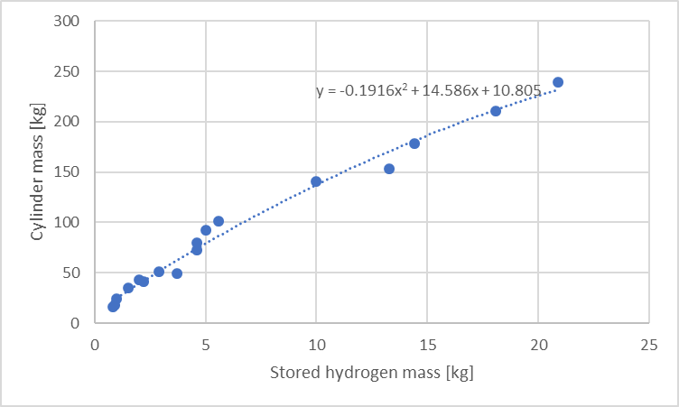
Figure 10: Relation between stored hydrogen mass and hydrogen storage cylinder mass
Note
Important remark: a battery is also added to fuel cell electric trucks. Based on manufacturer’s specification, its storage capacity represents approximately 6% of the storage capacity of the hydrogen cylinders, with a minimum of 20 kWh.
Charging stations
The parameters for the fast charging station used for battery electric trucks are presented in Table 16. The number of vehicles serviced by the charging station daily is defined by the battery capacity of the vehicles it serves. Theoretically, level-3 chargers can fast-charge the equivalent of 2’100 kWh daily, if operated within a safe SoC amplitude, or about five trucks with a 350 kWh battery pack.
EV charger, level 3, plug-in |
|
Vehicle type |
BEV-depot |
Power [kW] |
200 |
Efficiency [%] |
95 |
Source for efficiency |
|
Lifetime [years] |
24 |
Number of trucks allocated per charging system |
2’100 [kWh/day] / energy storage cap. [kWh] |
Share of the charging station allocated to the vehicle |
1 / (24 [years] * no. trucks * annual mileage [km/day] * cargo mass [ton]) |
Source for inventories |
|
Comment |
Assumed lifetime of 24 years. It is up scaled to represent a 200 kW Level-3 charger by scaling the charger component up based on a mass of 1’290 kg given by AAB’s 200 kW bus charger. |
Finding solutions
Very much like carculator and carculator_bus,
carculator_truck iterates on the sizing procedure until:
The change in curb mass of the vehicles between two modeling iterations is below 1%. This indicates that the vehicle model and the size of its components have stabilized, and further iterating will not affect its mass or its fuel consumption.
All while considering the following constraints:
For all trucks, the driving mass when fully occupied cannot be superior to the gross mass of the vehicle (this is specifically relevant for battery electric vehicles)
Particularly relevant to battery electric vehicles, the curb mass (including the battery mass) should be so low as to allow it to retain at least 10% of the initial cargo carrying capacity, all while staying under the permissible gross weight limit.
Validation
Diesel trucks
Figure 11 compares the fuel economy of trucks of different size classes
modeled by carculator_truck with those found in HBEFA and ecoinvent v.3.
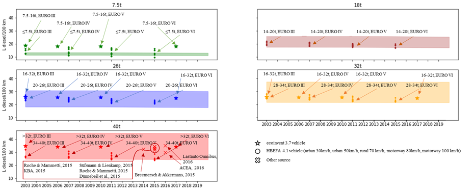
Figure 11: Fuel consumption for diesel trucks in L diesel per 100 km, against literature data.
Note
Shaded areas: the upper bound is calculated with the “Urban delivery” driving cycle with a load factor of 80%, the lower bound is calculated with the “Long haul” driving cycle with a load factor of 20%.
Battery electric trucks
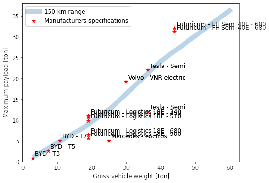
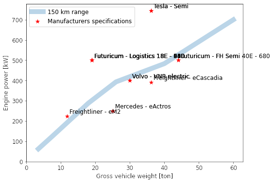
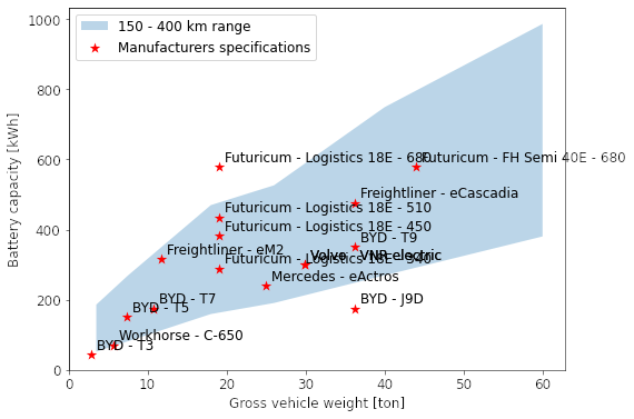
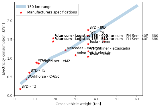
Table 17 compares some of the modeled parameters for battery electric trucks with the specifications of some commercial models disclosed by manufacturers. These manufacturers’ specifications can also be found in Annexes.
|
Maximum payload modeled (shaded line) versus commercial models, function of gross weight |
|
Engine peak power output modeled (shaded line) versus commercial models, function of gross weight |
|
Battery capacity modeled (shared area) versus commercial models, function of gross weight. The lower bound of the shaded area represents a vehicle with a range autonomy of 150 km. The upper bound of the shaded area represent a vehicle a range autonomy of 400 km. |
|
Tank-to-wheel energy consumption modeled (shaded line) versus commercial models, function of gross weight |
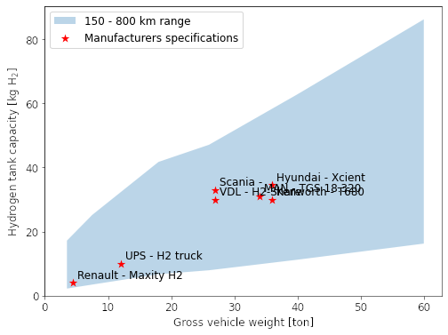
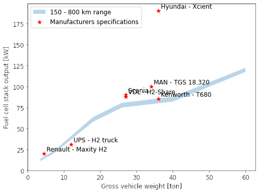
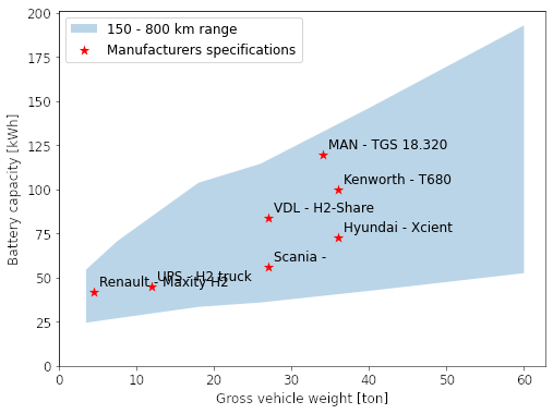
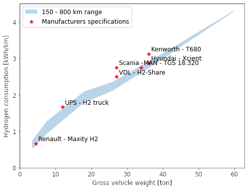
Fuel cell electric trucks
|
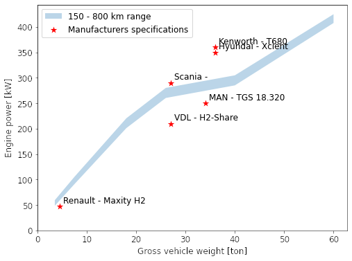
Engine peak power output modeled (shaded line) versus commercial models, function of gross weight |
|
Hydrogen tank capacity modeled (shaded line) versus commercial models, function of gross weight. The lower bound of the shaded area represents a vehicle with a range autonomy of 150 km. The upper bound of the shaded area represent a vehicle a range autonomy of 800 km. |
|
Fuel cell stack power output modeled (shaded line) versus commercial models, function of gross weight. |
|
Battery capacity modeled (shaded line) versus commercial models, function of gross weight. The lower bound of the shaded area represents a vehicle with a range autonomy of 150 km. The upper bound of the shaded area represent a vehicle a range autonomy of 800 km. |
|
Tank-to-wheel energy consumption modeled (shaded line) versus commercial models, function of gross weight. |
Inventory modelling
Once the vehicles are modeled, the calculated parameters of each of them is passed to the inventory.py calculation module to derive inventories. When the inventories for the vehicle and the transport are calculated, they can be normalized by the kilometric lifetime (i.e., vehicle-kilometer) or by the kilometric multiplied by the passenger occupancy (i.e., passenger-kilometer).
Road demand
The demand for construction and maintenance of roads and road-related infrastructure is calculated on the following basis:
Road construction: 5.37e-7 meter-year per kg of vehicle mass per km.
Road maintenance: 1.29e-3 meter-year per km, regardless of vehicle mass.
The driving mass of the vehicle consists of the mass of the vehicle in running condition (including fuel) in addition to the mass of passengers and cargo, if any. Unless changed, the passenger mass is 75 kilograms, and the average occupancy is 1.6 persons per vehicle.
The demand rates used to calculate the amounts required for road construction and maintenance (based on vehicle mass per km and per km, respectively) are taken from [Spielmann and Scholz, 2005].
Because roads are maintained by removing surface layers older than those that are actually discarded, road infrastructure disposal is modeled in ecoinvent as a renewal rate over the year in the road construction dataset.
Fuel properties
For all vehicles with an internal combustion engine, carbon dioxide (CO2) and sulfur dioxide (SO2) emissions are calculated based on the fuel consumption of the vehicle and the carbon and sulfur concentration of the fuel observed in Switzerland and Europe. Sulfur concentration values are sourced from HBEFA 4.1 [Benedikt and others, 2019]. Lower heating values and CO2 emission factors for fuels are sourced from p.86 and p.103 of [for the Environment, 2021]. The fuel properties shown in Table 19 are used for fuels purchased in Switzerland but should be applicable for other areas/countries.
Volumetric mass density [kg/l] |
Lower heating value [MJ/kg] |
CO2 emission factor [kg CO2/kg] |
SO2 emission factor [kg SO2/kg] |
|
|---|---|---|---|---|
Diesel |
0.85 |
43 |
3.15 |
8.85e-4 |
Biodiesel |
0.85 |
38 |
2.79 |
8.85e-4 |
Synthetic diesel |
0.85 |
43 |
3.15 |
0 |
Natural gas |
47.5 |
2.68 |
||
Bio-methane |
47.5 |
2.68 |
||
Synthetic methane |
47.5 |
2.68 |
Note
Note that carculator_truck will adapt the sulfur concentration of the
fuel (and related SOx emissions) based on the country the user selects (see Figure 12).
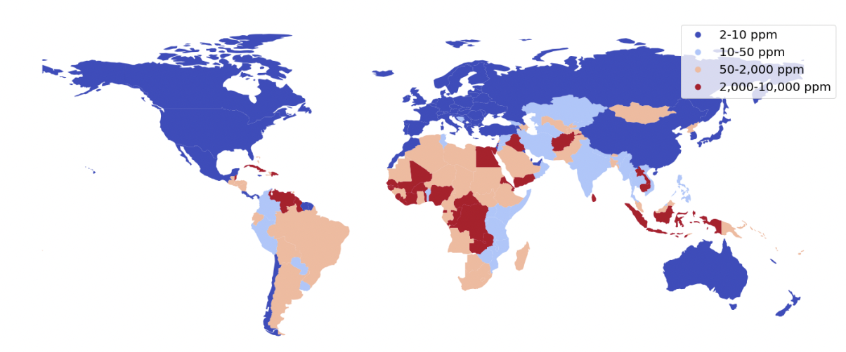
Figure 12: Region-specific sulfur concentration of diesel fuel. Source [Xie and others, 2020, Miller and Jin, 2019]
Exhaust emissions
Emissions of regulated and non-regulated substances during driving are approximated using emission factors from HBEFA 4.1 [Benedikt and others, 2019]. Emission factors are typically given in gram per km. Emission factors representing free flowing driving conditions and urban and rural traffic situations are used. Additionally, cold start emissions as well as running, evaporation and diurnal losses are accounted for, also sourced from HBEFA 4.1 [Benedikt and others, 2019].
For vehicles with an internal combustion engine, the sulfur concentration values in the fuel can slightly differ across regions - although this remains rather limited within Europe. The values provided by HBEFA 4.1 are used for Switzerland, France, Germany, Austria and Sweden. For other countries, values from [Miller and Jin, 2019] are used.
Sulfur [ppm/fuel wt.] |
Switzerland |
Europe |
|---|---|---|
Diesel |
10 |
8 |
The amount of sulfur dioxide released by the vehicle over one km [kg/km] is calculated as:
where \(r_{S}\) is the sulfur content per kg of fuel [kg SO2/kg fuel], \(F_{fuel}\) is the fuel consumption of the vehicle [kg/km], and \(64/32\) is the ratio between the molar mass of SO2 and the molar mass of O2.
Country-specific fuel blends are sourced from the IEA’s Extended World Energy Balances database [(IEA), 2021]. By default, the biofuel used is assumed to be produced from biomass residues (i.e., second-generation fuel): fermentation of crop residues for bioethanol, esterification of used vegetable oil for biodiesel and anaerobic digestion of sewage sludge for bio-methane.
Biofuel share [% wt.] |
Switzerland |
Europe |
|---|---|---|
Diesel blend |
4.8 |
6 |
Compressed gas blend |
22 |
9 |
For exhaust emissions, factors based on the fuel consumption are derived by comparing emission data points for different traffic situations (i.e., grams emitted per vehicle-km) for in a free flowing driving situation, with the fuel consumption corresponding to each data point (i.e., MJ of fuel consumed per km), as illustrated in Figure 12 for a diesel-powered engine. The aim is to obtain emission factors expressed in grams of substance emitted per MJ of fuel consumed, to be able to model emissions of passenger cars of different sizes and fuel efficiency and for different driving cycles.
Hence, the emission of substance i at second s of the driving cycle is calculated as follows:
where:
\(E(i,s)\) is the emission of substance i at second s of the driving cycle,
\(F_ttw(s)\) is the fuel consumption of the vehicle at second s,
and \(X(i, e)\) is the emission factor of substance i in the given driving conditions.
NMHC speciation
After NMHC emissions are quantified, EEA/EMEP’s 2019 Air Pollutant Emission Inventory Guidebook provides factors to further specify some of them into the substances listed in Table 22.
Trucks and buses (diesel) |
|
|---|---|
Wt. % of NMVOC |
|
Ethane |
0.03 |
Propane |
0.1 |
Butane |
0.15 |
Pentane |
0.06 |
Hexane |
0 |
Cyclohexane |
0 |
Heptane |
0.3 |
Ethene |
0 |
Propene |
0 |
1-Pentene |
0 |
Toluene |
0.01 |
m-Xylene |
0.98 |
o-Xylene |
0.4 |
Formaldehyde |
8.4 |
Acetaldehyde |
4.57 |
Benzaldehyde |
1.37 |
Acetone |
0 |
Methyl ethyl ketone |
0 |
Acrolein |
1.77 |
Styrene |
0.56 |
NMVOC, unspecified |
81.3 |
Non-exhaust emissions
A number of emission sources besides exhaust emissions are considered. They are described in the following sub-sections.
Engine wear emissions
Metals and other substances are emitted during the combustion of fuel because of engine wear. These emissions are scaled based on the fuel consumption, using the emission factors listed in Table 23, sourced from [Agency, 2019].
Trucks (diesel) |
|
|---|---|
kg/MJ fuel |
|
PAH |
1.82E-09 |
Arsenic |
2.33E-12 |
Selenium |
2.33E-12 |
Zinc |
4.05E-08 |
Copper |
4.93E-10 |
Nickel |
2.05E-10 |
Chromium |
6.98E-10 |
Chromium VI |
1.40E-12 |
Mercury |
1.23E-10 |
Cadmium |
2.02E-10 |
Abrasion emissions
We distinguish four types of abrasion emissions, besides engine wear emissions:
brake wear emissions: from the wearing out of brake drums, discs and pads
tires wear emissions: from the wearing out of rubber tires on the asphalt
road wear emissions: from the wearing out of the road pavement
and re-suspended road dust: dust on the road surface that is re-suspended as a result of passing traffic, “due either to shear forces at the tire/road surface interface, or air turbulence in the wake of a moving vehicle” [Beddows and Harrison, 2021].
[Beddows and Harrison, 2021] provides an approach for estimating the mass and extent of these abrasion emissions. They propose to disaggregate the abrasion emission factors presented in the EMEP’s 2019 Emission inventory guidebook [Agency, 2019] for two-wheelers, passenger cars, buses and heavy good vehicles, to re-quantify them as a function of vehicle mass, but also traffic situations (urban, rural and motorway). Additionally, they present an approach to calculate re-suspended road dust according to the method presented in [EPA, 2011] - such factors are not present in the EMEP’s 2019 Emission inventory guidebook - using representative values for dust load on European roads.
The equation to calculate brake, tire, road and re-suspended road dust emissions is the following:
With:
\(EF\) being the emission factor, in mg per vehicle-kilometer
\(W\) being the vehicle mass, in tons
\(b\) and \(c\) being regression coefficients, whose values are presented in Table 24.
Tire wear |
Brake wear |
Road wear |
Re-suspended road dust |
|||||||||||||
|---|---|---|---|---|---|---|---|---|---|---|---|---|---|---|---|---|
Urban |
Rural |
Motorway |
Urban |
Rural |
Motorway |
|||||||||||
b |
c |
b |
c |
b |
c |
b |
c |
b |
c |
b |
c |
b |
c |
b |
c |
|
PM 10 |
5.8 |
2.3 |
4.5 |
2.3 |
3.8 |
2.3 |
4.2 |
1.9 |
1.8 |
1.5 |
0.4 |
1.3 |
2.8 |
1.5 |
2 |
1.1 |
PM 2.5 |
8.2 |
2.3 |
6.4 |
2.3 |
5.5 |
2.3 |
11 |
1.9 |
4.5 |
1.5 |
1 |
1.3 |
5.1 |
1.5 |
8.2 |
1.1 |
The respective amounts of brake and tire wear emissions in urban, rural and motorway driving conditions are weighted, to represent the driving cycle used. The weight coefficients sum to 1 and the coefficients considered are presented in Table 25. They have been calculated by analyzing the speed profile of each driving cycle, with the exception of two-wheelers, for which no driving cycle is used (i.e., the energy consumption is from reported values) and where simple assumptions are made in that regard instead.
Driving cycle |
Urban |
Rural |
Motorway |
|
|---|---|---|---|---|
Truck, urban delivery |
Urban delivery |
1 |
||
Truck, regional delivery |
Regional delivery |
0.16 |
0.32 |
0.52 |
Truck, long haul |
Long haul |
1 |
Finally, for electric and (plugin) hybrid vehicles (with the exception of two-wheelers), the amount of brake wear emissions is reduced. This reduction is calculated as the ratio between the sum of energy recuperated by the regenerative braking system and the sum of negative resistance along the driving cycle. The logic is that the amount of negative resistance that could not be met by the regenerative braking system needs to be met with mechanical brakes.
Driving cycle |
Reduction factor for hybrid vehicles |
Reduction factor for plugin hybrid vehicles |
Reduction factor for battery and fuel cell electric vehicles |
|
|---|---|---|---|---|
Truck, urban delivery |
Urban delivery |
-20% |
-82% |
-82% |
Truck, regional delivery |
Regional delivery |
-24% |
-82% |
-83% |
The sum of PM 2.5 and PM 10 emissions is used as the input for the ecoinvent v.3.x LCI datasets indicated in Table 27.
Tire wear |
Brake wear |
Road wear |
Re-suspended road dust |
|
|---|---|---|---|---|
Truck |
Tyre wear emissions, lorry |
Brake wear emissions, lorry |
Road wear emissions, lorry |
Finally, we assume that the composition of the re-suspended road dust is evenly distributed between brake, road and tire wear particles.
Figure 13 below shows the calculated abrasion emissions for trucks in mg per vehicle-kilometer, following the approach presented above. These amounts will differ across driving cycles. For example, the amount of brake wear emissions is higher for the urban delivery cycle than for the regional delivery cycle, because the urban delivery cycle has a higher share of braking events.
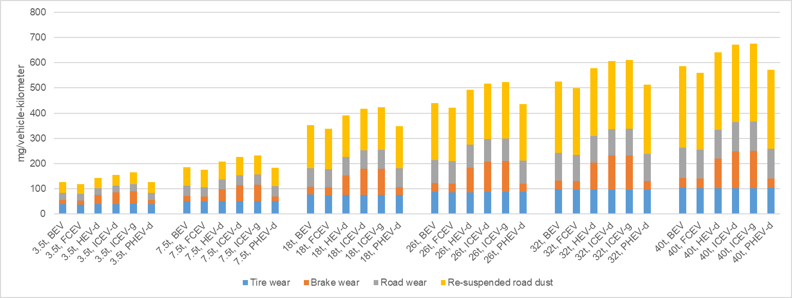
Figure 13: Total particulate matter emissions (<2.5 µm and 2.5-10 µm) in mg per vehicle-kilometer for trucks.
Refrigerant emissions
The use of refrigerant for onboard air conditioning systems is considered for trucks until 2021. The supply of refrigerant gas R134a is accounted for. Similarly, the leakage of the refrigerant is also considered. For this, the calculations from [P. and others, 2016] are used. Such emission is included in the transportation dataset of the corresponding vehicle. The overall supply of refrigerant amounts to the initial charge plus the amount leaked throughout the lifetime of the vehicle, both listed in Table 28. This is an important aspect, as the refrigerant gas R134a has a Global Warming potential of 2’400 kg CO2-eq./kg released in the atmosphere.
Trucks |
|
Initial charge [kg per vehicle lifetime] |
1.1 |
Lifetime loss [kg per vehicle lifetime] |
0.94 |
Note
Important assumption: it is assumed that electric and plug-in electric vehicles also use a compressor-like belt-driven air conditioning system, relying on the refrigerant gas R134a. In practice, an increasing, but still minor, share of electric vehicles now use a (reversible) heat pump to provide cooling.
Note
Important remark: After 2021, R134a is no longer used.
Noise emissions
Noise emissions along the driving cycle of the vehicle are quantified using the method developed within the CNOSSOS project [Kephalopoulos and others, 2012], which are expressed in joules, for each of the 8 octaves. Rolling and propulsion noise emissions are quantified separately.
The sound power level of rolling noise is calculated using:
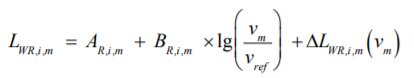
With:
\(v_m\) being the instant speed given by the driving cycle, in km/h
\(v_{ref}\) being the reference speed of 70 km/h
and \(A_{P,i,m}\) and \(B_{P,i,m}\) are unit-less and given in Table 29.
The propulsion noise level is calculated using:
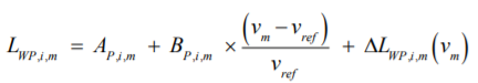
With:
\(v_m\) being the instant speed given by the driving cycle, in km/h
\(v_{ref}\) being the reference speed of 70 km/h
and \(A_{P,i,m}\) and \(B_{P,i,m}\) are unit-less and given in Table 29.
Octave band center frequency (Hz) |
AR |
BR |
AP |
BP |
|---|---|---|---|---|
63 |
84 |
30 |
101 |
-1.9 |
125 |
88.7 |
35.8 |
96.5 |
4.7 |
250 |
91.5 |
32.6 |
98.8 |
6.4 |
500 |
96.7 |
23.8 |
96.8 |
6.5 |
1000 |
97.4 |
30.1 |
98.6 |
6.5 |
2000 |
90.9 |
36.2 |
95.2 |
6.5 |
4000 |
83.8 |
38.3 |
88.8 |
6.5 |
8000 |
80.5 |
40.1 |
82.7 |
6.5 |
Octave band center frequency (Hz) |
AR |
BR |
AP |
BP |
|---|---|---|---|---|
63 |
87 |
30 |
104.4 |
0 |
125 |
91.7 |
33.5 |
100.6 |
3 |
250 |
94.1 |
31.3 |
101.7 |
4.6 |
500 |
100.7 |
25.4 |
101 |
5 |
1000 |
100.8 |
31.8 |
100.1 |
5 |
2000 |
94.3 |
37.1 |
95.9 |
5 |
4000 |
87.1 |
38.6 |
91.3 |
5 |
8000 |
82.5 |
40.6 |
85.3 |
5 |
A correction factor for battery electric and fuel cell electric vehicles is applied, and is sourced from [Pallas and others, 2016]. Also, electric vehicles are added a warning signal of 56 dB at speed levels below 20 km/h. Finally, hybrid vehicles are assumed to use an electric engine up to a speed level of 30 km/h, beyond which the combustion engine is used.
The total noise level (in A-weighted decibels) is calculated using the following equation:
The total sound power level is converted into Watts (or joules per second), using the following equation:
The total sound power, for each second of the driving cycle, is then distributed between the urban, suburban and rural inventory emission compartments.
Typically, propulsion noise emissions dominate in urban environments, thereby justifying the use of electric vehicles in that regard. Rolling noise become dominant above 50 km/h. The sound power [W] over time is expressed in joules [or W.s] over the course of the driving cycle.
The study from [Stefano and others, 2019] provides compartment-specific noise emission characterization factors against midpoint and endpoint indicators - expressed in Person-Pascal-second and Disability-Adjusted Life Year, respectively.
Electricity mix calculation
Electricity supply mix are calculated based on the weighting from the
distribution the lifetime kilometers of the vehicles over the years of
use. For example, should a BEV enter the fleet in Poland in 2020, most
LCA models of trucks would use the electricity mix for
Poland corresponding to that year, which corresponds to the row of the
year 2020 in Table 31, based on ENTSO-E’s TYNDP 2020 projections
(National Trends scenario) [ENTSO-E, 2020]. carculator_truck calculates instead the
average electricity mix obtained from distributing the annual kilometers
driven along the vehicle lifetime, assuming an equal number of
kilometers is driven each year. Therefore, with a lifetime of 200,000 km
and an annual mileage of 12,000 kilometers, the projected electricity
mixes to consider between 2020 and 2035 for Poland are shown in Table 31.
Using the kilometer-distributed average of the projected mixes
between 2020 and 2035 results in the electricity mix presented in the
last row of Table 31. The difference in terms of technology contribution
and unitary GHG-intensity between the electricity mix of 2020 and the
electricity mix based on the annual kilometer distribution is
significant (-23%). The merit of this approach ultimately depends on
whether the projections will be realized or not.
It is also important to remember that the unitary GHG emissions of each electricity-producing technology changes over time, as the background database ecoinvent has been transformed by premise [Sacchi and others, 2022]: for example, photovoltaic panels become more efficient, as well as some of the combustion-based technologies (e.g., natural gas). For more information about the transformation performed on the background life cycle database, refer to [Sacchi and others, 2022].
Year |
Biomass |
Coal |
Gas |
Gas CCGT |
Gas CHP |
Hydro |
Hydro, reservoir |
Lignite |
Nuclear |
Oil |
Solar |
Waste |
Wind |
Wind, offshore |
g CO2-eq./kWh |
|---|---|---|---|---|---|---|---|---|---|---|---|---|---|---|---|
2020 |
3% |
46% |
2% |
3% |
0% |
3% |
1% |
29% |
3% |
0% |
0% |
0% |
9% |
0% |
863 |
2021 |
2% |
43% |
2% |
4% |
1% |
3% |
1% |
29% |
2% |
0% |
1% |
3% |
9% |
0% |
841 |
2022 |
2% |
41% |
1% |
5% |
1% |
3% |
1% |
28% |
2% |
0% |
2% |
5% |
9% |
0% |
807 |
2023 |
1% |
38% |
1% |
5% |
2% |
2% |
1% |
28% |
1% |
0% |
3% |
8% |
10% |
0% |
781 |
2024 |
1% |
36% |
0% |
6% |
2% |
2% |
0% |
27% |
1% |
0% |
3% |
11% |
10% |
0% |
745 |
2025 |
0% |
33% |
0% |
7% |
3% |
2% |
0% |
27% |
0% |
0% |
4% |
13% |
10% |
0% |
724 |
2026 |
0% |
31% |
0% |
8% |
3% |
2% |
0% |
25% |
0% |
0% |
5% |
13% |
11% |
2% |
684 |
2027 |
0% |
28% |
0% |
9% |
4% |
2% |
0% |
24% |
0% |
0% |
6% |
12% |
12% |
3% |
652 |
2028 |
0% |
25% |
0% |
9% |
5% |
2% |
0% |
23% |
0% |
0% |
6% |
12% |
13% |
5% |
614 |
2029 |
0% |
23% |
0% |
10% |
6% |
2% |
0% |
21% |
0% |
0% |
7% |
11% |
14% |
6% |
580 |
2030 |
0% |
20% |
0% |
11% |
6% |
2% |
0% |
20% |
0% |
0% |
8% |
10% |
15% |
8% |
542 |
2031 |
0% |
19% |
0% |
11% |
7% |
2% |
0% |
18% |
1% |
0% |
9% |
10% |
16% |
8% |
514 |
2032 |
0% |
17% |
0% |
10% |
8% |
2% |
0% |
16% |
3% |
0% |
9% |
9% |
17% |
9% |
470 |
2033 |
0% |
16% |
0% |
10% |
8% |
2% |
0% |
14% |
4% |
0% |
10% |
8% |
17% |
10% |
437 |
2034 |
0% |
15% |
0% |
10% |
9% |
2% |
0% |
12% |
5% |
0% |
10% |
8% |
18% |
11% |
408 |
2035 |
0% |
13% |
0% |
9% |
10% |
2% |
0% |
11% |
7% |
0% |
11% |
7% |
19% |
12% |
377 |
Mix |
0% |
26% |
0% |
7% |
5% |
2% |
0% |
21% |
2% |
0% |
6% |
8% |
13% |
5% |
668 |
Inventories for fuel pathways
A number of inventories for fuel production and supply are used by
carculator_truck. They represent an update in comparison to the inventories
used in the passenger vehicles model initially published by [Brian and others, 2020].
The fuel pathways presented in Table 32 are from the literature
and not present as generic ecoinvent datasets.
Author(s) |
Fuel type |
Description |
|---|---|---|
Biodiesel from micro-algae |
2nd and 3rd generation biofuels made from biomass residues or algae. |
|
Biodiesel from used cooking oil |
||
e-Diesel (Fischer-Tropsch) |
Diesel produced from “blue crude” via a Fischer-Tropsch process. The H2 is produced via electrolysis, while the CO2 comes from direct air capture. Note that two allocation approaches at the crude-to-fuel step are possible between the different co-products (i.e., diesel, naphtha, wax oil, kerosene): energy or economic. |
|
Bio-methane from sewage sludge |
Methane produced from the anaerobic digestion of sewage sludge. The biogas is upgraded to bio-methane (the CO2 is separated and vented out) to a vehicle grade quality. |
|
Synthetic methane |
Methane produced via an electrochemical methanation process, with H2 from electrolysis and CO2 from direct air capture. |
|
Hydrogen from electrolysis |
The electricity requirement to operate the electrolyzer changes over time: from 58 kWh per kg of H2 in 2010, down to 44 kWh in 2050, according to [Christian and others, 2021]. |
|
Hydrogen from Steam Methane Reforming |
Available for natural gas and bio methane, with and without Carbon Capture and Storage (CCS). |
|
Hydrogen from woody biomass gasification |
Available with and without Carbon Capture and Storage (CCS). |
Inventories for energy storage components
The source for the inventories used to model energy storage components are listed in Table 33.
Author(s) |
Energy storage type |
Description |
|---|---|---|
NMC-111/622/811 battery |
Originally from [Qiang and others, 2019], then updated and integrated in ecoinvent v.3.8 (with some errors), corrected and integrated in the library. Additionally, these inventories relied exclusively on synthetic graphite. This is has too been modified: the anode production relies on a 50:50 mix of natural and synthetic graphite, as it seems to be the current norm in the industry [James and Dan, 2019]. Inventories for natural graphite are from [Engels et al., 2022]. |
|
NCA battery |
||
LFP battery |
||
Type IV hydrogen tank, default |
Carbon fiber being one of
the main components of
Type IV storage tanks,
new inventories for
carbon fiber
manufacturing have been
integrated to
|
|
Type IV hydrogen tank, LDPE liner |
||
Type IV hydrogen tank, aluminium liner |
Life cycle impact assessment
To build the inventory of every vehicle, carculator_truck populates a
three-dimensional array A (i.e., a tensor) such as:
The second and third dimensions (i.e., M and N) have the same length. They correspond to product and natural flow exchanges between supplying activities (i.e., M) and receiving activities (i.e., N). The first dimension (i.e., L) stores model iterations. Its length depends on whether the analysis is static or if an uncertainty analysis is performed (e.g., Monte Carlo).
Given a final demand vector f (e.g., 1 kilometer driven with a
specific vehicle, represented by a vector filled with zeroes and the
value 1 at the position corresponding to the index j of the driving
activity in dimension M) of length equal to that of the second dimension
of A (i.e., M), carculator_truck calculates the scaling factor s so
that:
Finally, the scaling factor s is multiplied with a characterization matrix B. This matrix contains midpoint characterization factors for a number of impact assessment methods (as rows) for every activity in A (as columns).
As described earlier, the tool chooses between several characterization matrices B, which contain pre-calculated values for activities for a given year, depending on the year of production of the vehicle as well as the REMIND climate scenario considered (i.e., “SSP2-Baseline”, “SSP2-PkBudg1150” or “SSP2-PkBudg500”). Midpoint and endpoint (i.e., human health, ecosystem impacts and resources use) indicators include those of the ReCiPe 2008 v.1.13 impact assessment method, as well as those of ILCD 2018. Additionally, it is possible to export the inventories in a format compatible with the LCA framework Brightway2 or SimaPro, thereby allowing the characterization of the results against a larger number of impact assessment methods.